From r to Q*: Your Language Model is Secretly a Q-Function

Motivation: $log\frac{\pi_{\theta}(y_i|[x, y^{<i}])} { \pi_{ref}(y_i|[x, y^{<i}])}$ 是否可以等价于第i个token的reward？

先放出DPO的优化目标： $max_{\pi_{\theta}}\mathbb{E}_{x\sim \mathcal{D}, y\sim \pi_{\theta}}[r_{\phi}(x,y)]-\beta\mathbb{D}_{KL}[\pi_{\theta}(y|x)\parallel \pi_(y|x)]$ 通过上式子的闭式解带入BT-model得到DPO最终的Loss为： $\mathcal{L} = -\mathbb{E}_{(x, y_w, y_l)}[\log\sigma(\beta\log \frac{\pi_{\theta}(y_w|x)}{\pi_{ref}(y_w|x)} - \beta\log \frac{\pi_{\theta}(y_l|x)}{\pi_{ref}(y_l|x)}))]$

在上一篇论文DPO中我们讲过可以简单地将整个回答看成是一个action，LLM执行一个action直接拿到一个sequence score。

DPO和核心的代码如下：

def preference_loss(policy_chosen_logps: torch.FloatTensor,
                    policy_rejected_logps: torch.FloatTensor,
                    reference_chosen_logps: torch.FloatTensor,
                    reference_rejected_logps: torch.FloatTensor,
                    beta: float,
                    label_smoothing: float = 0.0,
                    ipo: bool = False,
                    reference_free: bool = False) -> Tuple[torch.FloatTensor, torch.FloatTensor, torch.FloatTensor]:
    """Compute the DPO loss for a batch of policy and reference model log probabilities.

    Args:
        policy_chosen_logps: Log probabilities of the policy model for the chosen responses. Shape: (batch_size,)
        policy_rejected_logps: Log probabilities of the policy model for the rejected responses. Shape: (batch_size,)
        reference_chosen_logps: Log probabilities of the reference model for the chosen responses. Shape: (batch_size,)
        reference_rejected_logps: Log probabilities of the reference model for the rejected responses. Shape: (batch_size,)
        beta: Temperature parameter for the DPO loss, typically something in the range of 0.1 to 0.5. We ignore the reference model as beta -> 0.
        label_smoothing: conservativeness for DPO loss, which assumes that preferences are noisy (flipped with probability label_smoothing)
        ipo: If True, use the IPO loss instead of the DPO loss.
        reference_free: If True, we ignore the _provided_ reference model and implicitly use a reference model that assigns equal probability to all responses.

    Returns:
        A tuple of three tensors: (losses, chosen_rewards, rejected_rewards).
        The losses tensor contains the DPO loss for each example in the batch.
        The chosen_rewards and rejected_rewards tensors contain the rewards for the chosen and rejected responses, respectively.
    """
    pi_logratios = policy_chosen_logps - policy_rejected_logps
    ref_logratios = reference_chosen_logps - reference_rejected_logps

    if reference_free:
        ref_logratios = 0

    logits = pi_logratios - ref_logratios  # also known as h_{\pi_\theta}^{y_w,y_l}

    if ipo:
        losses = (logits - 1/(2 * beta)) ** 2  # Eq. 17 of https://arxiv.org/pdf/2310.12036v2.pdf
    else:
        # Eq. 3 https://ericmitchell.ai/cdpo.pdf; label_smoothing=0 gives original DPO (Eq. 7 of https://arxiv.org/pdf/2305.18290.pdf)
        losses = -F.logsigmoid(beta * logits) * (1 - label_smoothing) - F.logsigmoid(-beta * logits) * label_smoothing

    chosen_rewards = beta * (policy_chosen_logps - reference_chosen_logps).detach()
    rejected_rewards = beta * (policy_rejected_logps - reference_rejected_logps).detach()

    return losses, chosen_rewards, rejected_rewards

# 以下是logps的计算函数，默认average_log_prob=False
def _get_batch_logps(logits: torch.FloatTensor, labels: torch.LongTensor, average_log_prob: bool = False) -> torch.FloatTensor:
    """Compute the log probabilities of the given labels under the given logits.

    Args:
        logits: Logits of the model (unnormalized). Shape: (batch_size, sequence_length, vocab_size)
        labels: Labels for which to compute the log probabilities. Label tokens with a value of -100 are ignored. Shape: (batch_size, sequence_length)
        average_log_prob: If True, return the average log probability per (non-masked) token. Otherwise, return the sum of the log probabilities of the (non-masked) tokens.

    Returns:
        A tensor of shape (batch_size,) containing the average/sum log probabilities of the given labels under the given logits.
    """
    assert logits.shape[:-1] == labels.shape

    labels = labels[:, 1:].clone()
    logits = logits[:, :-1, :]
    loss_mask = (labels != -100)

    # dummy token; we'll ignore the losses on these tokens later
    labels[labels == -100] = 0

    per_token_logps = torch.gather(logits.log_softmax(-1), dim=2, index=labels.unsqueeze(2)).squeeze(2)

    if average_log_prob:
        return (per_token_logps * loss_mask).sum(-1) / loss_mask.sum(-1)
    else:
        return (per_token_logps * loss_mask).sum(-1)

从上面实际代码可以看出计算DPO损失时，因为y本身也是一个序列，序列出现的概率为每一个$y_i$的概率的乘积，因此： $\log(\pi(y|x)) = \sum_{i=1}^{N}\log(\pi(y^i|x))$ 带入DPO的Loss公式，得到： $\mathcal{L} = -\mathbb{E}_{(x, y_w, y_l)}[\log\sigma(\beta \sum_{i=1}^{N_1}\log\frac{\pi_{\theta}(y_w^i|[x, y_w^{<i}])}{\pi_{ref}(y_w^i|[x, y_w^{<i}])} - \beta\sum_{i=1}^{N_2}\log\frac{\pi_{\theta}(y_l^i|[x, y_l^{<i}])}{\pi_{ref}(y_l^i|[x, y_l^{<i}])}))]$ 看起来貌似是一个“token-level”的reward，但是在原来的DPO理论分析中并没有体现出来，于是我们在思考，假如我们从token reward的角度去分析DPO，那么是不是会有新的发现呢？ 比如每一个token的reward是不是可以看成$\log\frac{\pi_{\theta}(y_t|[x, y_w^i])}{\pi_{ref}(y_t|[x, y_w^i])}$？答案是肯定的，但是这个推导并不trival。

Soft Q learning框架 + DPO

既然是token level reward了，那么最优化的目标也需要进行改写，下式中的$s_t=[x, y^{<t}]$代表的是x和y中前t-1个token的concatenation： $\begin{aligned} &\ \ \ \ \max_{\theta}\mathbb{E}_{x\sim \mathcal{D}, y\sim \pi_{\theta}}[\sum_{t=1}^{T}r(s_t, y_t)]-\beta\mathbb{D}_{KL}[\pi_{\theta}(y|x)\parallel \pi_{ref}(y|x)]\\ &=\max_{\theta}\mathbb{E}_{x\sim \mathcal{D}, y\sim \pi_{\theta}}\Big[\sum_{t=1}^{T}[r(s_t, y_t)+\beta\log\pi_{ref}(y_t|s_t) + \beta H(\pi_{\theta}(s_t))]\Big] \end{aligned}$ 将$r(s_t, y_t)+\beta\log\pi_{ref}(y_t|s_t)$看成$r'(s_t, y_t)$，不考虑数据集上的期望x，考虑某一个具体的样本x，那么优化目标可以写成： $\max_{\theta}\sum_{t=1}^{T}\mathbb{E}_{y_t\sim \pi_{\theta}(s_t)}\Big[r'(s_t, y_t)+\beta H(\pi_{\theta}(s_t))\Big]$

仔细一看这个目标，不正是Soft Q learning的Mat Ent RL的目标吗？

而根据SQL中的理论结果，最优策略必然会满足： $\pi_{\theta}^*(y_t|s_t) = \exp(\frac{1}{\beta} Q^*(s_t, y_t)-\frac{1}{\beta} V^*(s_t))$

其中 $Q^*(s_t, y_t)=r'(s_t, a_t)+\mathbb{E}_{\pi^*}\Big[\sum_{k=t+1}^T\Big(r'(s_k,y_k)+\beta H(\pi^*({s_{k}}))\Big)\Big]$ $V^*(s_t)=\beta\int\exp(\frac{1}{\beta}Q^*(s_t, y_t))dy_t$

按照最优解的方程，我们有如下性质：

• 性质1，直接从$Q^*$的定义式反递归展开得到： $Q^*(s_t, y_t) = r'(s_t, y_t) + \beta H(\pi^*(s_t))+ \mathbb{E}_{a_{t+1}\sim\pi^*(s_{t+1})}\Big[Q^*(s_{t+1}, y_{t+1})\Big]$
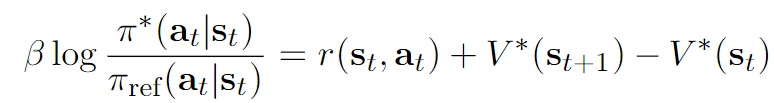
• 性质2： $Q^*(s_t, y_t) = r'(s_t, y_t) + V^*(s_{t+1})$ 证明： $\beta H(\pi^*(s_t))+ \mathbb{E}_{a_{t+1}\sim\pi^*(s_{t+1})}\Big[Q^*(s_{t+1}, y_{t+1})\Big]$展开即可得到$V^*(s_{t+1})$的定义式。

于是乎，我们得到了如下的$Q^*$的另外一种表达式： $Q^*(s_t, y_t)= \begin{cases} r(s_t, y_t) +\beta\log \pi_{ref}(y_t|s_t) + V^*(s_{t+1}) & \text{if } y_t \neq EOS\\ r(s_t, y_t) + \beta\log \pi_{ref}(y_t|s_t) & \text{if } y_t = EOS \end{cases}$

前面的推导其实完全是SQL中的若干公式的复写，而我们的最终目的是preference，所以还是需要将注意力回归到BT-model，而BT-model重心是$\sum_{t=1}^{T}r(s_t, y_t)$的sigmoid下的比较。

$\begin{aligned} \sum_{t=1}^{T}r(s_t, y_t) &= \sum_{t=1}^T\Big( Q(s_t, y_t) - \beta\log\pi_{ref}(y_t|x)-V(s_{t+1})\Big)\\ & = V^*(s_1) + \sum_{t=1}^T\beta\log\frac{\pi_{\theta}(y_t|x)}{\pi_{ref}(y_t|x)} \end{aligned}$

因此： $p_{\pi^*}(\tau_w>\tau_l) = \sigma\Big(\sum_{t=1}^{N}\beta\log\frac{\pi_{\theta}(y_t^w|s_t)}{\pi_{ref}(y_t^w|x)} - \sum_{t=1}^{M}\beta\log\frac{\pi_{\theta}(y_t^l|x)}{\pi_{ref}(y_t^l|x)} \Big)$

通过优化$p_{\pi^*}(\tau_w>\tau_l)$，我们其实将$\pi$往$\pi^*$靠拢。

但是问题又来了，我们这个推导完全没办法知道$r(s_t, a_t)$的具体形式，也就是说它并不一定等于$\beta\log\frac{\pi_{\theta}(y_t|x)}{\pi_{ref}(y_t|x)}$。只是说按照$Q^*$，$V^*$我们在计算$\sum_{t=1}^{T}r(s_t, y_t)$恰好得到$V^*(s_1) + \sum\beta\log\frac{\pi_{\theta}(y_t|x)}{\pi_{ref}(y_t|x)}$，然后这个$V^*(s_1)$在BT中被消掉了。

Reward shaping

第一个小节提出的问题是，为什么$r(s_t, y_t)$可以等价于$\beta\log\frac{\pi_{\theta}(y_t|s_t)}{\pi_{ref}(y_t|s_t)}$？

但是第二小节的推导又告诉我们，$r(s_t, y_t)$的形式不一定是$\beta\log\frac{\pi_{\theta}(y_t|s_t)}{\pi_{ref}(y_t|s_t)}$。

这一小节，我们从reward之间的等价性入手，说明使用$\log\frac{\pi_{\theta}(y_t|x)}{\pi_{ref}(y_t|x)}$作为token reward，与使用$r(s_t, y_t)$作为token reward得到的最优策略是一样的。