Diffuser: Planning with diffusion for flexible behavior synthesis
在阅读本文之前,请确保你对DDPM有比较详细的了解。
核心:
- 将整条轨迹看作DDPM中的一个样本点,实践中,一般选取某个固定长度的轨迹作为 Diffuser 的输入输出,即将轨迹作为 Diffuser 加噪去噪的对象
前向扩散过程通常预先通过某种规则进行定义,不含可学习参数。
去噪过程:
结构图如下:
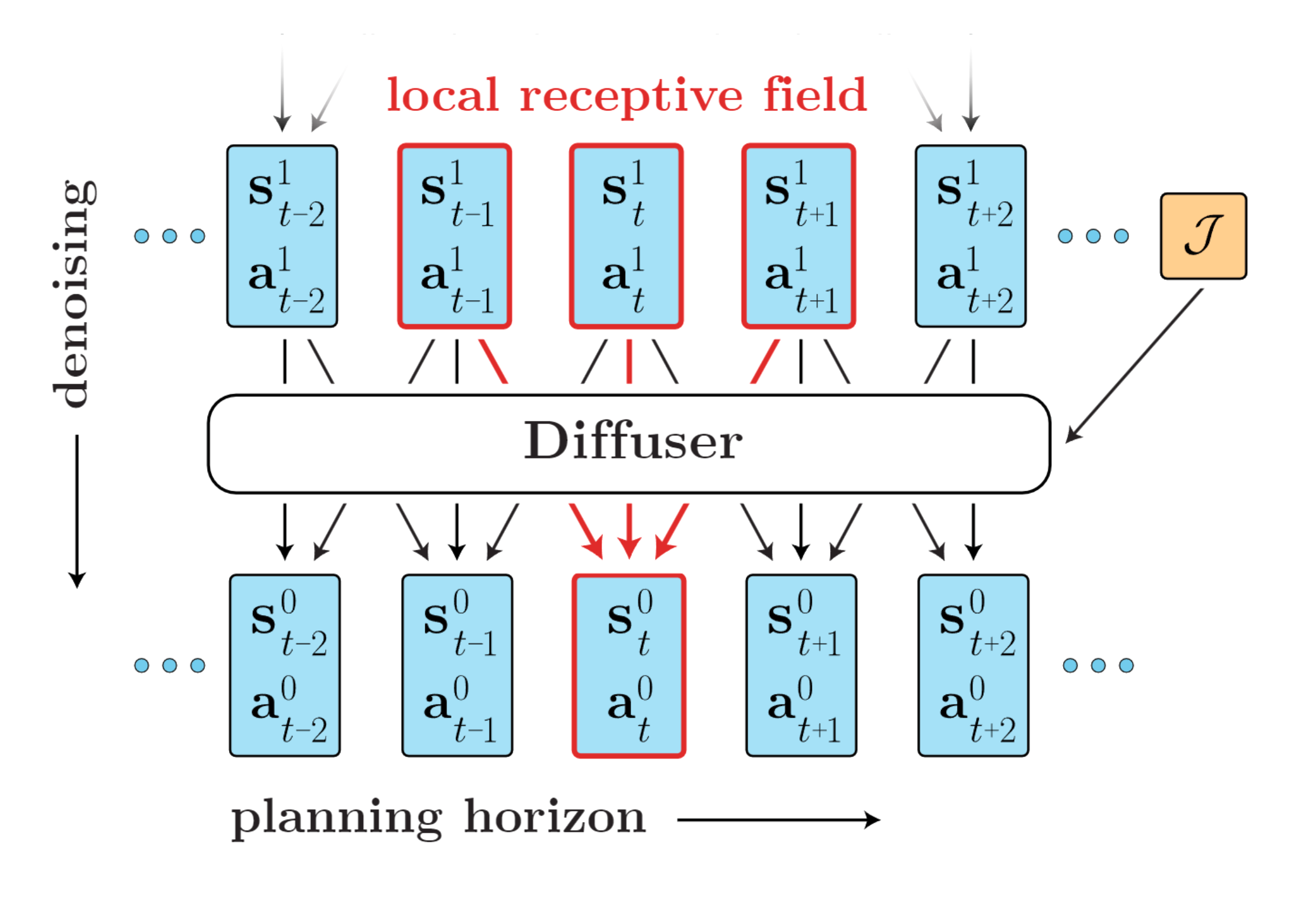
讲到这里,其实你只需要一个简单的理解方式,给定一个长度为的轨迹片段,我们获得一个图片,这个图片长度为,宽度为1,通道数为。DDPM处理的一般长宽均大于1的图片,正常用的是2D卷积的Unet,这里我们显然只需要用1D卷积的Unet就可以了。这也就是论文提到的Temporal locality(仔细想想一维的卷积就可以理解了,相邻时间步经过线性组合得到输出)
class GaussianDiffusion(nn.Module):
    def __init__(self, model, horizon, observation_dim, action_dim, n_timesteps=1000,
        loss_type='l1', clip_denoised=False, predict_epsilon=True,
        action_weight=1.0, loss_discount=1.0, loss_weights=None,
    ):
        super().__init__()
        self.horizon = horizon
        self.observation_dim = observation_dim
        self.action_dim = action_dim
        self.transition_dim = observation_dim + action_dim
        self.model = model

        betas = cosine_beta_schedule(n_timesteps)
        alphas = 1. - betas
        alphas_cumprod = torch.cumprod(alphas, axis=0)
        alphas_cumprod_prev = torch.cat([torch.ones(1), alphas_cumprod[:-1]])

        self.n_timesteps = int(n_timesteps)
        self.clip_denoised = clip_denoised
        self.predict_epsilon = predict_epsilon

        self.register_buffer('betas', betas)
        self.register_buffer('alphas_cumprod', alphas_cumprod)
        self.register_buffer('alphas_cumprod_prev', alphas_cumprod_prev)

        # calculations for diffusion q(x_t | x_{t-1}) and others
        self.register_buffer('sqrt_alphas_cumprod', torch.sqrt(alphas_cumprod))
        self.register_buffer('sqrt_one_minus_alphas_cumprod', torch.sqrt(1. - alphas_cumprod))
        self.register_buffer('log_one_minus_alphas_cumprod', torch.log(1. - alphas_cumprod))
        self.register_buffer('sqrt_recip_alphas_cumprod', torch.sqrt(1. / alphas_cumprod))
        self.register_buffer('sqrt_recipm1_alphas_cumprod', torch.sqrt(1. / alphas_cumprod - 1))

        # calculations for posterior q(x_{t-1} | x_t, x_0)
        posterior_variance = betas * (1. - alphas_cumprod_prev) / (1. - alphas_cumprod)
        self.register_buffer('posterior_variance', posterior_variance)

        ## log calculation clipped because the posterior variance
        ## is 0 at the beginning of the diffusion chain
        self.register_buffer('posterior_log_variance_clipped',
            torch.log(torch.clamp(posterior_variance, min=1e-20)))
        self.register_buffer('posterior_mean_coef1',
            betas * np.sqrt(alphas_cumprod_prev) / (1. - alphas_cumprod))
        self.register_buffer('posterior_mean_coef2',
            (1. - alphas_cumprod_prev) * np.sqrt(alphas) / (1. - alphas_cumprod))

        ## get loss coefficients and initialize objective
        loss_weights = self.get_loss_weights(action_weight, loss_discount, loss_weights)
        self.loss_fn = Losses[loss_type](loss_weights, self.action_dim)

    def get_loss_weights(self, action_weight, discount, weights_dict):
        '''
            sets loss coefficients for trajectory

            action_weight   : float
                coefficient on first action loss
            discount   : float
                multiplies t^th timestep of trajectory loss by discount**t
            weights_dict    : dict
                { i: c } multiplies dimension i of observation loss by c
        '''
        self.action_weight = action_weight

        dim_weights = torch.ones(self.transition_dim, dtype=torch.float32)

        ## set loss coefficients for dimensions of observation
        if weights_dict is None: weights_dict = {}
        for ind, w in weights_dict.items():
            dim_weights[self.action_dim + ind] *= w

        ## decay loss with trajectory timestep: discount**t
        discounts = discount ** torch.arange(self.horizon, dtype=torch.float)
        discounts = discounts / discounts.mean()
        loss_weights = torch.einsum('h,t->ht', discounts, dim_weights)

        ## manually set a0 weight
        loss_weights[0, :self.action_dim] = action_weight
        return loss_weights

    #------------------------------------------ sampling ------------------------------------------#

    def predict_start_from_noise(self, x_t, t, noise):
        '''
            if self.predict_epsilon, model output is (scaled) noise;
            otherwise, model predicts x0 directly
        '''
        if self.predict_epsilon:
            return (
                extract(self.sqrt_recip_alphas_cumprod, t, x_t.shape) * x_t -
                extract(self.sqrt_recipm1_alphas_cumprod, t, x_t.shape) * noise
            )
        else:
            return noise

    def q_posterior(self, x_start, x_t, t):
        posterior_mean = (
            extract(self.posterior_mean_coef1, t, x_t.shape) * x_start +
            extract(self.posterior_mean_coef2, t, x_t.shape) * x_t
        )
        posterior_variance = extract(self.posterior_variance, t, x_t.shape)
        posterior_log_variance_clipped = extract(self.posterior_log_variance_clipped, t, x_t.shape)
        return posterior_mean, posterior_variance, posterior_log_variance_clipped

    def p_mean_variance(self, x, cond, t):
        x_recon = self.predict_start_from_noise(x, t=t, noise=self.model(x, cond, t))

        if self.clip_denoised:
            x_recon.clamp_(-1., 1.)
        else:
            assert RuntimeError()

        model_mean, posterior_variance, posterior_log_variance = self.q_posterior(
                x_start=x_recon, x_t=x, t=t)
        return model_mean, posterior_variance, posterior_log_variance

    @torch.no_grad()
    def p_sample_loop(self, shape, cond, verbose=True, return_chain=False, sample_fn=default_sample_fn, **sample_kwargs):
        device = self.betas.device

        batch_size = shape[0]
        x = torch.randn(shape, device=device)
        x = apply_conditioning(x, cond, self.action_dim)

        chain = [x] if return_chain else None

        progress = utils.Progress(self.n_timesteps) if verbose else utils.Silent()
        for i in reversed(range(0, self.n_timesteps)):
            t = make_timesteps(batch_size, i, device)
            x, values = sample_fn(self, x, cond, t, **sample_kwargs)
            x = apply_conditioning(x, cond, self.action_dim)

            progress.update({'t': i, 'vmin': values.min().item(), 'vmax': values.max().item()})
            if return_chain: chain.append(x)

        progress.stamp()

        x, values = sort_by_values(x, values)
        if return_chain: chain = torch.stack(chain, dim=1)
        return Sample(x, values, chain)

    @torch.no_grad()
    def conditional_sample(self, cond, horizon=None, **sample_kwargs):
        '''
            conditions : [ (time, state), ... ]
        '''
        device = self.betas.device
        batch_size = len(cond[0])
        horizon = horizon or self.horizon
        shape = (batch_size, horizon, self.transition_dim)

        return self.p_sample_loop(shape, cond, **sample_kwargs)

    #------------------------------------------ training ------------------------------------------#

    def q_sample(self, x_start, t, noise=None):
        if noise is None:
            noise = torch.randn_like(x_start)

        sample = (
            extract(self.sqrt_alphas_cumprod, t, x_start.shape) * x_start +
            extract(self.sqrt_one_minus_alphas_cumprod, t, x_start.shape) * noise
        )

        return sample

    def p_losses(self, x_start, cond, t):
        noise = torch.randn_like(x_start)

        x_noisy = self.q_sample(x_start=x_start, t=t, noise=noise)
        x_noisy = apply_conditioning(x_noisy, cond, self.action_dim)

        x_recon = self.model(x_noisy, cond, t)
        x_recon = apply_conditioning(x_recon, cond, self.action_dim)

        assert noise.shape == x_recon.shape

        if self.predict_epsilon:
            loss, info = self.loss_fn(x_recon, noise)
        else:
            loss, info = self.loss_fn(x_recon, x_start)

        return loss, info

    def loss(self, x, *args):
        batch_size = len(x)
        t = torch.randint(0, self.n_timesteps, (batch_size,), device=x.device).long()
        return self.p_losses(x, *args, t)

    def forward(self, cond, *args, **kwargs):
        return self.conditional_sample(cond, *args, **kwargs)
你可能感疑惑,为什么里面有一个condition的处理,其实它是将轨迹的第一个状态永远作为已知内容,读完下面的图像修复的论文,或许你会对这件事情理解更加深刻。下面我们临时中断一下,插入一篇CVPR2022的论文。
RePaint: Inpainting using Denoising Diffusion Probabilistic Models
这里插入一个简短的CVPR2022论文介绍。
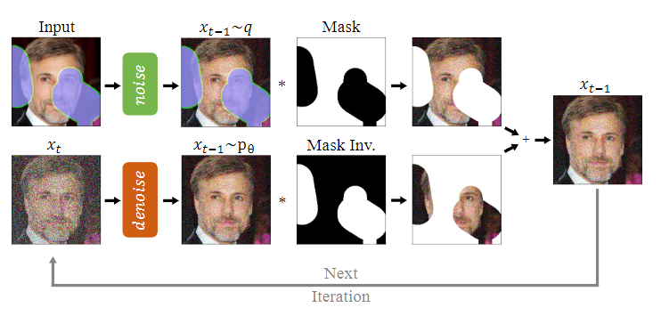
想解决的任务:图像修复。输入一张受损的图片,输出一个修复后的图片。本文只是一个采样方法,训练阶段跟DDPM保持一致。
任务:
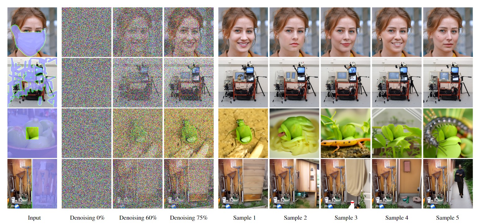
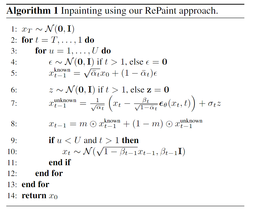
跟DDPM不一样的地方在于,DDPM训练完之后模型输入是高斯噪声,然后经过T步的reverse过程之后采样得到图片,但是在Repaint里面,一开始是有一张受损的图片的,所以我们需要把这个信息用上,具体用的方法是使用mask(假设已知哪块区域受损需要修复),如下图所示:
个人代码讲解
链接:https://pan.baidu.com/s/1WXohoYheETVKKmuNKCl4BQ?pwd=scy6
提取码:scy6
The full trajectory of state-action pairs form a single sample for the diffusion model. A separate return model is learned to predict the cumulative rewards of each trajectory sample. The guidance of the return model is then injected into the reverse sampling stage. This approach is similar to Decision Transformer, which also learns a trajectory generator through GPT2 with the help of the true trajectory returns. When used online, sequence models can no longer predict actions from states autoregressively (since the states are an outcome of the environment). Thus, in the evaluation stage, a whole trajectory is predicted for each state while only the first action is applied, which incurs a large computational cost.
某种程度上,Diffuser跟model-based有点类似,只是dynamics和policy同时学习(from model-based trajectory-planning),所以Diffuser属于Diffusion+RL里面的Planner一类的算法。
下面是伟楠老师的Diffusion Models for Reinforcement Learning: A Survey的对这一类算法的描述,我觉得讲的非常好:
Planning in RL refers to using a dynamic model to make decisions imaginarily and selecting the appropriate action to maximize cumulative rewards. This process usually explores various sequences of actions and states, thus improving decisions over a longer horizon. Planning is commonly used in the MBRL framework with a learned dynamic model. However, the planning sequences are usually simulated autoregressively, which may lead to severe compounding errors, especially in the offline setting due to limited data support. Diffusion models offer a promising alternative as they can generate multi-step planning sequences simultaneously.