CQL: Conservative Q-Learning for Offline Reinforcement Learning
CQL算是质量非常高的论文了,个人觉得是理论和实验完美适配的论文,而且行文流畅,是不可多得的佳作。但是代码实现上不是太容易,相比于之后我们会讲的IQL,虽然IQL的理论性稍微差了一点,但是从实验效果和代码实现上来看,IQL更容易上手。
一作Aviral Kumar也是D4RL的作者。
CQL的基本思想:从Q值上进行约束,对于那些ood的Q值进行打压。
符号约定
CQL的符号很多,想要读懂这篇论文,首先得进入这篇论文的符号体系。
Online RL下的符号约定
这些符号与CQL这篇论文无关了,主要是为了让读者熟悉一下RL中的一些基本符号。
: Transition function, 表示在状态下,执行动作后,得到的下一个状态是的概率。
: Reward function, 表示在状态下,执行动作后,得到的reward。
: Policy, 表示在状态下,执行动作的概率。
: Bellman Equation, 称B为贝尔曼迭代算子,
策略迭代分为两个步骤:策略评估和策略改进。策略评估就是求解Bellman Equation,策略改进就是让策略朝着更好的方向更新。
策略评估:
策略改进:
注意到该贝尔曼算子依赖于策略,Q和V值的近似与策略相关,最后Q和V的收敛值也与策略相关。常见的Actor-Critic算法都属于这个系列。
Offline RL下的符号约定
首先是数据集,我们假设是由一个行为策略采集得到的,是一个确定性策略,是策略的参数。当然实际数据集还可能是多个策略采集得到的数据的混合,此时行为策略为多个策略之间的加权。
通常来说,数据集的大小是有限的,因此定义经验分布: 经验分布是对行为策略的一个经验估计,当足够大时,会收敛到。
类似地,我们定义真实环境转移概率,表示在状态下,Agent执行动作后,得到的下一个状态是的概率。我们也可以定义经验估计。其计算方式是类似的:
同理,我们可以定义真实reward函数和经验估计。总之,离线数据集其实对应了一个经验MDP,OfflineRL中,我们使用这个经验MDP来进行训练得到最终的策略。
所有加上\hat{}的符号都是经验估计,代表着对真实值的一个经验估计。
当离线数据集给定时,、、都是确定的,分别代表了行为策略、状态转移概率、reward的经验估计。实际操作中我们并不会直接按照前面的定义式计算这些值。
类似于前面的Online RL的“两步走”,我们可以给出一个naive版本的策略学习方案: 策略评估:
策略改进:
其中,策略评估的写法完全等价于:
所有符号总结如下:
| 符号 | 含义 |
|---|---|
| offline dataset | |
| behavioral policy, 也就是offline dataset中的行为策略,数据集由这个策略采集得到 | |
| 经验分布函数,是对的一个经验估计, | |
| 下,Agent执行后,得到的的真实状态转移概率 | |
| 下,Agent执行后,得到的的经验估计的状态转移概率 | |
| 下,Agent执行后,得到的reward | |
| 下,Agent执行后,得到的reward的经验估计, | |
我们在这里先简单介绍一些后面会用到的等式和不等式。
- 第一个性质:
证明:
刨除(s, a),,收敛时: 等价于:
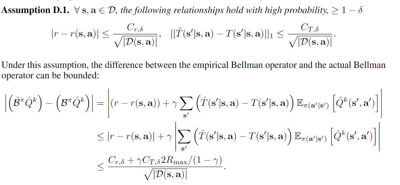
第二个性质:
在特定假设下,我们的经验贝尔曼算子和真实贝尔曼算子满足以下关系:

naive版本的核心代码
这一小节我们实现一个naive版本的算法,相比于上一小节的推导,我们多了一个entropy的约束,所有的估计得到的都是\hat{}的值。和通过迭代最终收敛。
dataset = d4rl.qlearning_dataset(env)
replayer_buffer = ReplayBuffer(dataset)

...
batch = replayer_buffer.sample_batch(batch_size)
dict = agent.update(batch)

    def update(self, data_batch):
        (
            obs_batch,
            action_batch,
            reward_batch,
            next_obs_batch,
            done_batch,
            truncated_batch,
        ) = itemgetter("obs", "action", "reward", "next_obs", "done", "truncated")(
            data_batch
        )

        reward_batch = reward_batch * self.reward_scale

        # calculate critic loss
        curr_q1 = self.q1_network([obs_batch, action_batch])
        curr_q2 = self.q2_network([obs_batch, action_batch])
        with torch.no_grad():
            next_obs_action, next_obs_log_prob = itemgetter("action", "log_prob")(
                self.policy_network.sample(next_obs_batch)
            )

            target_q1_value = self.target_q1_network([next_obs_batch, next_obs_action])
            target_q2_value = self.target_q2_network([next_obs_batch, next_obs_action])
            next_obs_min_q = torch.min(target_q1_value, target_q2_value)
            target_q = next_obs_min_q - self.alpha * next_obs_log_prob
            target_q = reward_batch + self.gamma * (1.0 - done_batch) * target_q

        # compute q loss and backward
        q1_loss = F.mse_loss(curr_q1, target_q)
        q2_loss = F.mse_loss(curr_q2, target_q)

        self.q1_optimizer.zero_grad()
        self.q2_optimizer.zero_grad()

        ##########

        new_curr_obs_action, new_curr_obs_log_prob = itemgetter("action", "log_prob")(
            self.policy_network.sample(obs_batch)
        )
        new_curr_obs_q1_value = self.q1_network([obs_batch, new_curr_obs_action])
        new_curr_obs_q2_value = self.q2_network([obs_batch, new_curr_obs_action])
        new_min_curr_obs_q_value = torch.min(
            new_curr_obs_q1_value, new_curr_obs_q2_value
        )
        # compute policy and ent loss
        policy_loss = (
            (self.alpha * new_curr_obs_log_prob) - new_min_curr_obs_q_value
        ).mean()
        if self.automatic_entropy_tuning:
            alpha_loss = -(
                self.log_alpha * (new_curr_obs_log_prob + self.target_entropy).detach()
            ).mean()
            alpha_loss_value = alpha_loss.detach().cpu().item()
            self.alpha_optim.zero_grad()
        else:
            alpha_loss = 0.0
            alpha_loss_value = 0.0

        self.policy_optimizer.zero_grad()
        (policy_loss + alpha_loss).backward()
        self.policy_optimizer.step()
        if self.automatic_entropy_tuning:
            self.alpha_optim.step()
            self.alpha = self.log_alpha.detach().exp()

        self.update_target_network()

        return {
            "loss/q1": q1_loss.item(),
            "loss/q2": q2_loss.item(),
            "loss/policy": policy_loss.item(),
            "loss/entropy": alpha_loss_value,
            "misc/entropy_alpha": self.alpha.item(),
            "misc/lagrange_alpha": (
                self.log_lagrange_alpha.detach().exp().item()
                if self.with_lagrange
                else 0
            ),
        }
CQL的核心思想:打压action ood的Q值
这个章节的思路基本上按照原论文的Section3 The Conservative Q-Learning (CQL) Framework 来写。
action ood问题在BCQ中已经提到过了,简单来说,就是因为很有可能会导致没有出现在dataset里面,即完全是不准的,直接的后果便是的更新目标是不准的。我们称之为action的ood(out-of-distribution)问题。
简单的打压方式如下,我们简单称为(1):
这里的是一个一般化的写法,代表一个任意的策略。对比一下前面的navie的版本,我们实际上在做一个trade-off:一方面希望Q按照贝尔曼方程进行更新,另一方面通过约束Q值不要太大,从而达到“打压”的目的。
但是这样的优化会带来一个毛病,就是打压过于严重了,本来我们只是想打压那些ood的Q值,但是这样的优化会导致所有的Q值都被打压。所以,我们放松了一点限制,对于出现在数据集的(s, a)对应的Q值,我们认为这些值的估计应该会比较准,因此我们尽量不进行打压,于是得到了如下的优化目标,我们称为(2):
我们断言,通过选取适当的的值,可以使得按照这种方式迭代收敛得到的,这样就达到了我们的目的。下面两个定理告诉我们,我们前面定义的两种“打压”方式是有效果的(看不懂很正常,后面理论分析章节再详细的看看)。
所有的理论分析我们放到最后面,我们只讲大概的idea。
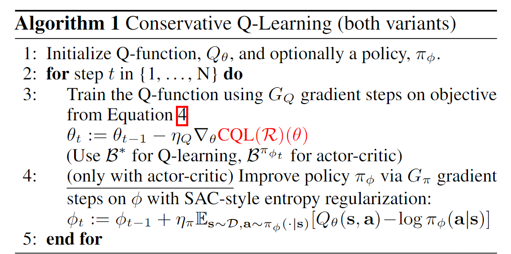
好了,我们现在手里头策略评估也就是更新Q值的方式用的是(2)。
其中一般是一个regularization term,比如熵正则化或者KL散度正则化(相比于某一个策略)。
实际优化过程中,因为仅仅只是进行一次随机梯度下降,所以未必会收敛到上式的最优,因此我们会使用以下的优化目标作为(2)式的实际目标:
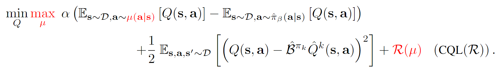
我们嵌套了两层,内层的最大化能够确保最优的,其对应的是的解(这样其实刚好是的最优)。
你可能会好奇:咦,弄了两层的优化有什么好处,看起来不是更加复杂了吗?
非也非也,我们再来看一下策略优化过程中的目标:
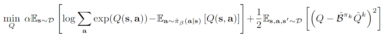
如果即最大化熵,那么毫无疑问,我们的策略最优解就是我们的玻尔兹曼分布:
于是最优化的同时:
因此,最终我们策略评估的损失:

代码实现
class CQLAgent(BaseAgent):
def __init__(
self,
observation_space,
action_space,
target_smoothing_tau,
alpha,
reward_scale,
# CQL specific
num_random_action_selection,
min_q_weight,
temp,
with_lagrange, # Defaults to true
lagrange_thresh,
**kwargs
):
super(CQLAgent, self).__init__()
obs_shape = observation_space.shape
self.action_space = action_space
# initilize networks
if isinstance(action_space, gym.spaces.box.Box):
self.discrete_action_space = False
action_dim = action_space.shape[0]
if len(observation_space.shape) == 1:
self.q1_network = SequentialNetwork(
obs_shape[0] + action_dim, 1, **kwargs["q_network"]
)
self.q2_network = SequentialNetwork(
obs_shape[0] + action_dim, 1, **kwargs["q_network"]
)
self.target_q1_network = SequentialNetwork(
obs_shape[0] + action_dim, 1, **kwargs["q_network"]
)
self.target_q2_network = SequentialNetwork(
obs_shape[0] + action_dim, 1, **kwargs["q_network"]
)
elif len(observation_space.shape) == 3:
raise NotImplementedError
else:
assert 0, "unsopprted observation_space"
else:
assert 0, "unsupported action space for CQL"
self.policy_network = PolicyNetworkFactory.get(
observation_space, action_space, **kwargs["policy_network"]
)
# sync network parameters
functional.soft_update_network(self.q1_network, self.target_q1_network, 1.0)
functional.soft_update_network(self.q2_network, self.target_q2_network, 1.0)
# pass to util.device
self.q1_network = self.q1_network.to(util.device)
self.q2_network = self.q2_network.to(util.device)
self.target_q1_network = self.target_q1_network.to(util.device)
self.target_q2_network = self.target_q2_network.to(util.device)
self.policy_network = self.policy_network.to(util.device)
# initialize optimizer
self.q1_optimizer = get_optimizer(
kwargs["q_network"]["optimizer_class"],
self.q1_network,
kwargs["q_network"]["learning_rate"],
)
self.q2_optimizer = get_optimizer(
kwargs["q_network"]["optimizer_class"],
self.q2_network,
kwargs["q_network"]["learning_rate"],
)
self.policy_optimizer = get_optimizer(
kwargs["policy_network"]["optimizer_class"],
self.policy_network,
kwargs["policy_network"]["learning_rate"],
)
# entropy
self.automatic_entropy_tuning = kwargs["entropy"]["automatic_tuning"]
self.alpha = alpha
if self.automatic_entropy_tuning:
self.target_entropy = -np.prod(
action_space.shape
).item() # 连续熵的话,因为每一个dim[-1, 1]对应的熵为log(b-a) = 1,所以总的熵为dim * 1
self.log_alpha = torch.zeros(1, requires_grad=True, device=util.device)
self.alpha = self.log_alpha.detach().exp()
self.alpha_optim = torch.optim.Adam(
[self.log_alpha], lr=kwargs["entropy"]["learning_rate"]
)
# hyper-parameters
self.gamma = kwargs["gamma"]
self.target_smoothing_tau = target_smoothing_tau
self.reward_scale = reward_scale
self.num_random_action_selection = num_random_action_selection
self.min_q_weight = min_q_weight
self.temp = temp
self.with_lagrange = with_lagrange
self.lagrange_thresh = lagrange_thresh
if self.with_lagrange:
self.target_action_gap = lagrange_thresh # \tau
self.log_lagrange_alpha = torch.zeros(
1, requires_grad=True, device=util.device
)
self.log_lagrange_alpha_optim = torch.optim.Adam(
[self.log_lagrange_alpha], lr=kwargs["q_network"]["learning_rate"]
)
def update(self, data_batch):
(
obs_batch,
action_batch,
reward_batch,
next_obs_batch,
done_batch,
truncated_batch,
) = itemgetter("obs", "action", "reward", "next_obs", "done", "truncated")(
data_batch
)
reward_batch = reward_batch * self.reward_scale
# calculate critic loss
curr_q1 = self.q1_network([obs_batch, action_batch])
curr_q2 = self.q2_network([obs_batch, action_batch])
with torch.no_grad():
next_obs_action, next_obs_log_prob = itemgetter("action", "log_prob")(
self.policy_network.sample(next_obs_batch)
)
target_q1_value = self.target_q1_network([next_obs_batch, next_obs_action])
target_q2_value = self.target_q2_network([next_obs_batch, next_obs_action])
next_obs_min_q = torch.min(target_q1_value, target_q2_value)
target_q = next_obs_min_q - self.alpha * next_obs_log_prob
target_q = reward_batch + self.gamma * (1.0 - done_batch) * target_q
# compute q loss and backward
q1_loss = F.mse_loss(curr_q1, target_q)
q2_loss = F.mse_loss(curr_q2, target_q)
self.q1_optimizer.zero_grad()
self.q2_optimizer.zero_grad()
##########
# above is the same as the sac agent, below is the cql part
batch_size = obs_batch.shape[0]
action_dim = action_batch.shape[-1]
# [batch_size * num_random_action_selection, action_dim] from action space
random_uniform_actions = (
torch.FloatTensor(
batch_size * self.num_random_action_selection,
action_dim,
)
.uniform_(-1, 1) # default action space is [-1, 1]
.to(util.device)
)
# the probability density of the uniform distribution is 1/(b-a), so log prob is -log(b-a), since each action is independent, so the log prob is the sum of each action's log prob
random_uniform_log_pi = np.log(0.5**action_dim)
obs_repeat = (
obs_batch.unsqueeze(1)
.repeat(1, self.num_random_action_selection, 1)
.view(-1, obs_batch.shape[-1])
) # [batch_size * num_random_action_selection, obs_dim]
next_obs_repeat = (
next_obs_batch.unsqueeze(1)
.repeat(1, self.num_random_action_selection, 1)
.view(-1, next_obs_batch.shape[-1])
)
q1_random = self.q1_network([obs_repeat, random_uniform_actions]).view(
batch_size, self.num_random_action_selection, 1
)
q2_random = self.q2_network([obs_repeat, random_uniform_actions]).view(
batch_size, self.num_random_action_selection, 1
)
policy_sample_actions, policy_sample_log_prob = itemgetter(
"action", "log_prob"
)(self.policy_network.sample(obs_repeat, deterministic=False))
policy_sample_log_prob = policy_sample_log_prob.view(
batch_size, self.num_random_action_selection, 1
)
policy_sample_next_actions, policy_sample_next_log_prob = itemgetter(
"action", "log_prob"
)(self.policy_network.sample(next_obs_repeat, deterministic=False))
policy_sample_next_log_prob = policy_sample_next_log_prob.view(
batch_size, self.num_random_action_selection, 1
)
q1_current_policy = self.q1_network([obs_repeat, policy_sample_actions]).view(
batch_size, self.num_random_action_selection, 1
)
q2_current_policy = self.q2_network([obs_repeat, policy_sample_actions]).view(
batch_size, self.num_random_action_selection, 1
)
q1_next_policy = self.q1_network(
[next_obs_repeat, policy_sample_next_actions]
).view(batch_size, self.num_random_action_selection, 1)
q2_next_policy = self.q2_network(
[next_obs_repeat, policy_sample_next_actions]
).view(batch_size, self.num_random_action_selection, 1)
q1_items = torch.cat(
[
q1_random - random_uniform_log_pi,
q1_current_policy - policy_sample_log_prob.detach(),
q1_next_policy - policy_sample_next_log_prob.detach(),
],
dim=1,
)
q2_items = torch.cat(
[
q2_random - random_uniform_log_pi,
q2_current_policy - policy_sample_log_prob.detach(),
q2_next_policy - policy_sample_next_log_prob.detach(),
],
dim=1,
) # [batch_size, num_random_action_selection * 2, 1]
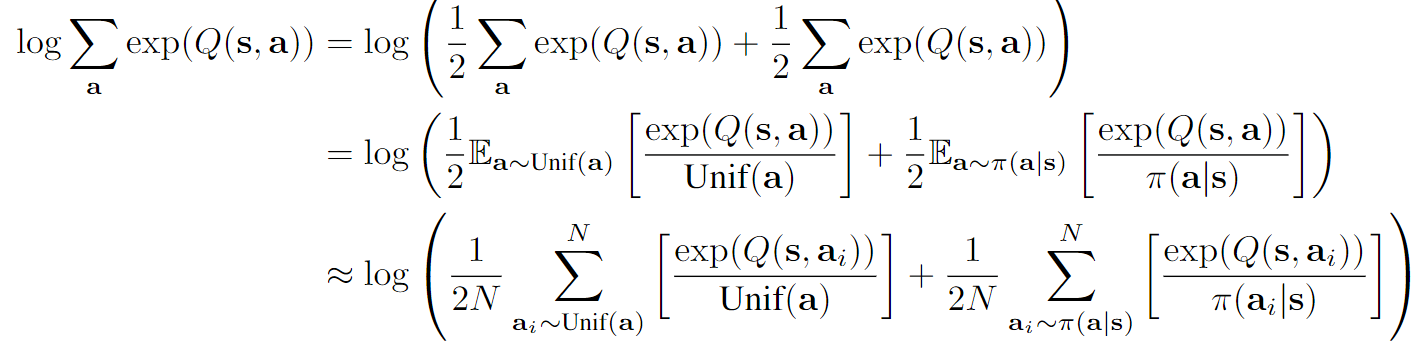
# logsumexp
q1_log_exp = torch.logsumexp(q1_items / self.temp, dim=1) * self.temp
q2_log_exp = torch.logsumexp(q2_items / self.temp, dim=1) * self.temp
q1_diff = self.min_q_weight * (q1_log_exp - curr_q1).mean()
q2_diff = self.min_q_weight * (q2_log_exp - curr_q2).mean()
if self.with_lagrange:
raise NotImplementedError
lagrange_alpha = torch.clamp(self.log_lagrange_alpha.exp(), 0, 1e6)
q1_log_exp = lagrange_alpha * (q1_log_exp - self.target_action_gap)
q2_log_exp = lagrange_alpha * (q2_log_exp - self.target_action_gap)
self.log_lagrange_alpha_optim.zero_grad()
alpha_loss = (-q1_log_exp - q2_log_exp) * 0.5
alpha_loss.backward(retain_graph=True)
self.log_lagrange_alpha_optim.step()
(q1_loss + q2_loss + q1_diff + q2_diff).backward()
self.q1_optimizer.step()
self.q2_optimizer.step()
##########
new_curr_obs_action, new_curr_obs_log_prob = itemgetter("action", "log_prob")(
self.policy_network.sample(obs_batch)
)
new_curr_obs_q1_value = self.q1_network([obs_batch, new_curr_obs_action])
new_curr_obs_q2_value = self.q2_network([obs_batch, new_curr_obs_action])
new_min_curr_obs_q_value = torch.min(
new_curr_obs_q1_value, new_curr_obs_q2_value
)
# compute policy and ent loss
policy_loss = (
(self.alpha * new_curr_obs_log_prob) - new_min_curr_obs_q_value
).mean()
if self.automatic_entropy_tuning:
alpha_loss = -(
self.log_alpha * (new_curr_obs_log_prob + self.target_entropy).detach()
).mean()
alpha_loss_value = alpha_loss.detach().cpu().item()
self.alpha_optim.zero_grad()
else:
alpha_loss = 0.0
alpha_loss_value = 0.0
self.policy_optimizer.zero_grad()
(policy_loss + alpha_loss).backward()
self.policy_optimizer.step()
if self.automatic_entropy_tuning:
self.alpha_optim.step()
self.alpha = self.log_alpha.detach().exp()
self.update_target_network()
return {
"loss/q1": q1_loss.item(),
"loss/q2": q2_loss.item(),
"loss/policy": policy_loss.item(),
"loss/entropy": alpha_loss_value,
"misc/entropy_alpha": self.alpha.item(),
"misc/lagrange_alpha": (
self.log_lagrange_alpha.detach().exp().item()
if self.with_lagrange
else 0
),
}
def update_target_network(self):
functional.soft_update_network(
self.q1_network, self.target_q1_network, self.target_smoothing_tau
)
functional.soft_update_network(
self.q2_network, self.target_q2_network, self.target_smoothing_tau
)
@torch.no_grad()
def select_action(self, obs, deterministic=False):
if len(obs.shape) in [1, 3]:
obs = [obs]
if type(obs) != torch.tensor:
obs = torch.FloatTensor(np.array(obs)).to(util.device)
action, log_prob = itemgetter("action", "log_prob")(
self.policy_network.sample(obs, deterministic=deterministic)
)
if self.discrete_action_space:
action = action[0]
return {"action": action.detach().cpu().numpy(), "log_prob": log_prob[0]}
官方实验结果:
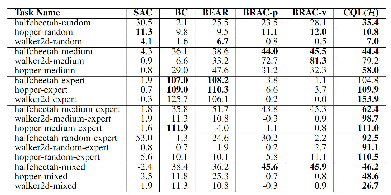
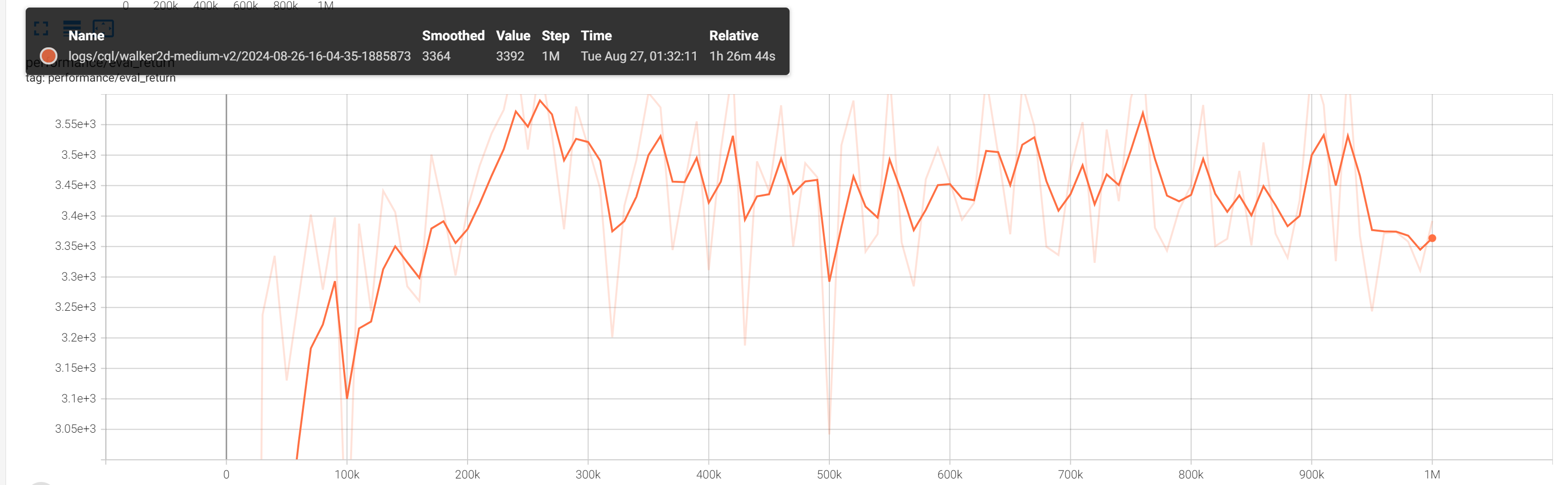
我自己并没有把实验都跑了,只是尝试了几个,并且也没有选取多个种子,只是确保代码基本逻辑没问题就没有深究了:
- Walker2D-medium-v2 的实验结果:
部分理论分析
OK,接下来就是比较硬核的环节了,我们需要对前面的两个定理Theorem 3.1和Theorem 3.2进行证明。先声明一下,这个小节并不是一板一眼的证明,对论文的定理的理解也不要试图一行一行的读,而是先看懂大方向想表达什么意思,再从骨架上给出证明。
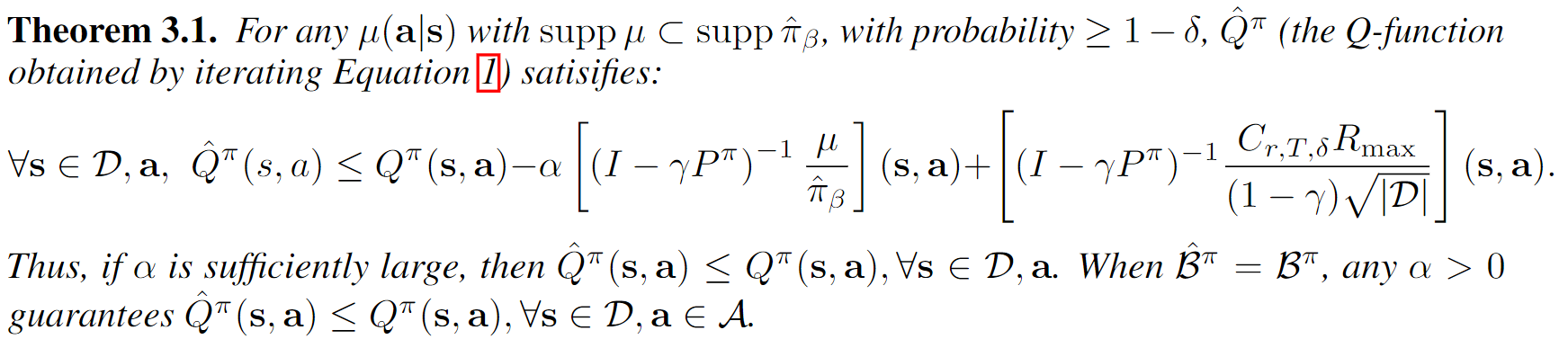
Theorem 3.1
我们先用人话描述一下定理3.1的内容: 通过(1)优化收敛得到的经验Q值与真实环境中经过真实贝尔曼迭代优化得到的Q值的差值被某一个界bound住,并且只要超参数精心设计,那么bound可以=0,即我们不会存在Q值高估的问题。即“打压”有效,我们不会高估Q值。证明如下:
对(1)求导,并令导数为0,我们得到(这个应该不难吧):
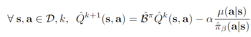
显而易见的一个结论是:。不过这个结论后面没用上,只是说看起来我们确实是在“打压”Q值,多减去。
考虑到我们在最前面提到的真实贝尔曼算子和经验贝尔曼算子之间的关系:
我们可以得到(感觉论文写得不太对,不过这个按照这个绝对值不等式展开再带入应该是不难得到的):

最终,我们有:
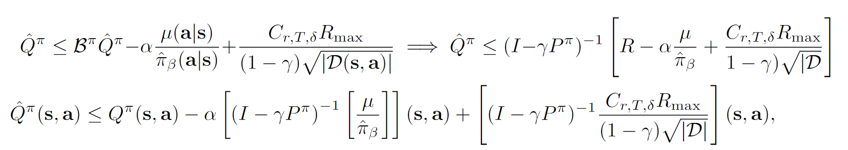
ok,这个推导相对麻烦一点(但是也不是很难):
因为,带入左上方第一个不等式,移动项目即可以得到右上方的不等式。
再注意到我们在最前面提到的第一个性质: 。
结合这个性质带入我们的不等式就可以得到最终的结果了。
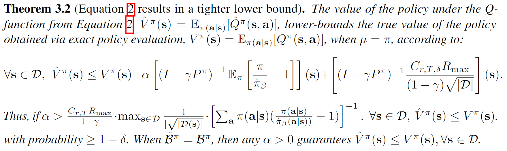
Theorem 3.2
TBD